Spatially Expanding Hierarchical Trees for Compliant Multi-Dimensional Scaling

Thomas Rebotier,

Interactive Cognition Laboratory,

University of California, San Diego

Abstract:

This article suggests a new type of initial configuration to use for gradient descent multidimensional scaling algorithms such as the Kruskal-Shepard algorithm. Using a binary hierarchical tree of the points to scale, one can expand that tree in the final space, starting with the root and repeatedly replacing each node by its two successors; at each expansion one uses the gradient descent again to reshape the configuration. Compared to applying gradient descent to the result of classical scaling, tree expansion yields similar levels of stress, but renders better the grouping of points belonging to similar clusters.

Introduction

When trying to visualize the proximity structure of a high dimensional pattern, one frequently has to choose between clustering into a hierarchical tree, or scaling down to two or three dimensions. Conventional wisdom considers that multi-dimensional scaling (MDS) is good at representing the big picture, whereas hierarchical clustering (HC) handles local details more accurately (Kruskal 1977; Arabie, Hubert et al. 1996). Ideally, one would want a low-dimensional configuration rendering both the global and local properties; such that, for example, if one drew between the final points a hierarchical tree obtained from the original data, this tree would appear simple and related branches would stay next to each other. This paper suggests a method that finds such tree-friendly scaling configurations.

There is a second situation where existing strategies come short: if there exists extraneous information in addition to the dissimilarities. For example, the points can be extracted from known different populations, such as male and female participants in an experiment, or different political parties in an opinion poll. The different clusters may or not have the same spatial distribution; yet of the many stress-equivalent ways of representing the data, some must better than others at representing this extraneous information. Likely, it is better to group together points belonging to the same cluster. In some cases, the preexisting classification may be hierarchical. For example, a library can display a 2-dimensional map of topics and sciences by scaling similarities between sciences; in which case it is important to respect the library’s call number system along with the similarity structure. Until now, both classical and non-metric scaling are ill-equipped to represent jointly the similarity structure and extraneous information. In contrast, the method suggested here can use such extraneous information.

Before we introduce our method, let us review the shortcomings of current MDS strategies. Consider a set of data points (P_i) of known dissimilarities (δ_i,j) that has to be visualized in two dimensions. When the dissimilarities should approximate directly actual distances between points, the MDS is metric, and can be done in two ways: by classical MDS, in which the points are projected orthogonally in the subspace encoding a maximum of variance (Young and Householder 1938; Torgerson 1952; Cox and Cox 2001), or by a metric gradient descent, trying to minimize the sum of residuals (the squared differences between distances and the corresponding dissimilarities). When the mapping between dissimilarities and distances is unknown—for example obscured by an unknown psychometric function—one can rely only on the order of the dissimilarities, and scaling is achieved by repeating a gradient descent trying to minimize the sum of residuals between distances and the same distances monotonically reduced to the dissimilarities (Shepard 1962; Shepard 1962; Kruskal 1964; Kruskal 1964). In the following paragraphs we will examine in turn why classical, metric MDS misrepresents smaller inter-point distances, and how gradient descent algorithms, including non-metric scaling, depend on initial configurations.

Why existing scaling strategies deal poorly with local structure:

1. In the case of classical multi-dimensional scaling (CMDS), the (δ_i,j)’s are taken to represent Euclidian distances, and (P_i) can be rendered after a Young-Torgerson reduction, by projecting the points in two dimensions for graphing (Young and Householder 1938; Torgerson 1952; Cox and Cox 2001). However, CMDS is not the best least squares rendering of distances– it is only the best rendering by orthogonal projection. In fact the sum of residuals (sum of squared error over inter-point distances) computed for a CMDS result is always high, in part because CMDS, like all orthogonal projections, systematically decreases distances. The following example (Figure 1) shows where problems can lie:

Figure 1: Classic MDS will project B and C onto the same point at intersection of dotted axes, but minimal least square error for the distances within a one-dimensional configuration is for B” and C”, whose center is at d_AB from A, and whose distance d_B”C” = d_BC/3.

Figure 1 illustrates two problems:

Because it lies parallel to an eigenvector pruned by the CMDS, the distance between B and C has been ignored. In contrast, the distance between A and the other points is almost conserved, because it is almost collinear to the eigenvector preserved by the CMDS.
The projection ignores the arc, so that even though B and C are both at the same distance from A, their projection gets closer than that distance.

A first step in estimating the true efficiency of CMDS is to dilate resulting distances by a factor ρ² = Σ_ij [(δ_ij.d_ij)/(d_ij²)]. This factor makes up for dividing the average arc by its cosine. Even then the sum of residuals can easily lag by 20% behind that obtained after a gradient descent adjustment (see the results section and Figure 5).

Still, CMDS reduces the original distances unequally, depending on which eigenvector bears most of a distance. For this reason, CMDS can mistreat gravely the details of local structure when these details lie in dimensions that are suppressed. When the algorithm deals with high-dimensional underlying patterns, it is very likely that many local patterns will be entirely misrepresented because of this CMDS shortcoming. So, if one wants to render as accurately as possible the set of between-point distances, CMDS projection must be followed by a gradient descent to minimize the sum of square errors.

However, even metric gradient descent starting from the CMDS configuration can fail to properly restitute local sub-patterns, because when the initial projection brings inside a 2-D sub-pattern points that should lie outside, the gradient descent is unable to move them outside, and the “pressure” caused by their presence distorts local details. This is illustrated below in Figure 2, where CMDS superimposes two clusters that should be kept separated, and gradient descent as a result explodes one of the clusters into a ring around the other one.

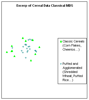
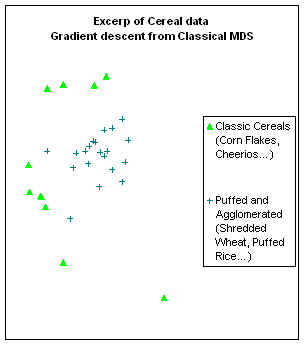
Figure 2: Detail of MDS made on the ASA Cereal data set. Two out of seven types of cereals are projected on top of each other by CMDS. Applying gradient descent worsens this particular feature of the configuration, because the central repulsion creates a crown of local minima in which the “classic cereal” points settle.

2. In the non-metric case, the (δ_ij) are on an ordinal rather than a ratio scale, in which case an initial configuration is modified to optimize the rank order of the resulting distances, (d_i,j). The Shepard-Kruskal algorithm (Shepard 1962; Shepard 1962; Kruskal 1964; Kruskal 1964) establishes for existing distances (d_ij) a set of target distances (d’_ij) that are in the same order as the (δ_ij)’s—when d_ij is already in order, d’_ij is set to equal d_ij,and when sequences of d_ij ’s are in disarray, all corresponding d’_ij ’s are set to the average of these d_ij,’s. The target distances are then used as dissimilarities in a metric gradient descent that modifies the initial configuration to minimize Stress (the normalized sum of residuals, Σ(d_ij-d’_ij)²/Σd_ij² ). Because this metric gradient descent can disturb the rank order again, the process must be iterated, until the configuration is stable.

Because gradient descent adjusts an initial configuration to a local minimum,its result depends on this initial configuration. To obtain a good final solution, one possible strategy is to try several random initial configurations and keep the most favorable. While this method in theory can explore the entire space of solutions, it is computationally costly. In practice a few attempts will generally yield at least one solution with acceptable stress. A second strategy is to use the result of CMDS as a starting configuration; this can be done after applying CMDS either on the dissimilarities themselves (treating them as distances), or on pseudo-distances reconstructed to be consistent with the rank order of dissimilarities (Lingoes and Roskam 1973). This latter strategy is a one-shot attempt, computationally effective but final. It can occasionally fail, as illustrated in Figure 3, and cannot be improved gracefully by increasing computational power. In conclusion, neither random configurations nor a CMDS-produced configuration are ideal starting points for the Kruskal-Shepard non-metric MDS.

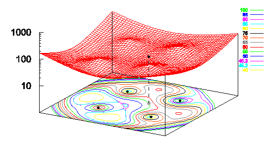
Figure 3: Local minima in a metric energy landscape and failure of CMDS-seeded gradient descent. When scaling the five points (4, 4, 0), (4,-4,0), (-4,4,0), (-4,-4,0) and (1,1,7), CMDS projects the latter in the plane Z=0, onto the point (1,1,0) shown in grey. This graph shows a 2-D section of a 10-variable function: the sum of residuals landscape, by fixing the coordinates of the 4 points that were already in the plane (“the base”) and showing the sum of residuals for different locations of the 5^th point. For moving the grey point only, there are at least five local minima: four located outside the base and one about (-1, -1, 0). In fact, this latter point is where gradient descent takes the grey point, but it is not the absolute minimum.

The tree-expansion strategy:

In summary, gradient descent appears as the best method to render the dissimilarities, but on one hand it requires a good starting configuration, and on the other hand it does not take in consideration the supplementary information that can be given by a hierarchical tree. We suggest solving these two problems together by using that supplementary information to construct a starting configuration which gradient descent will optimize with regard to stress. In the process of arranging the points (P_i) in two dimensions, the dissimilarity structure is unavoidably impoverished – but it can be impoverished less, by keeping in the final configuration some of the information obtained by a clustering algorithm, independently of the scaling algorithm.

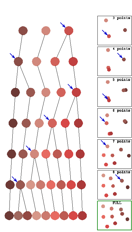
In order to jointly minimize stress and render the cluster structure, we propose to apply gradient descent (or Kruskal-Shepard) repeatedly to a growing configuration, obtained by expanding the hierarchical tree. This is illustrated by Figure 4 in which the hierarchical tree and successive configurations are shown bide by side. Prior to using this algorithm, one needs the dissimilarity matrix at all stages of expansion. If the tree has been constructed from a SAHN algorithm these dissimilarities are already available, otherwise they have to be computed in a one-sweep forward pass. Given these dissimilarities, the algorithm is to:

1. Position a starting configuration:

a. Take a section of the hierarchical tree containing D+1 points where D is the final dimension (e.g., 3 points for a planar MDS). This is the current section of the tree.

b. Using the dissimilarities between these points, place them in space exactly using CMDS.

c. Test that the resulting configuration defines a variety of dimension D. If yes, this is the starting configuration. If no, use as current section a section with one more point (the highest numbered tree node in the current section is replaced by its two offspring), and go to step b.

2. Expand the tree:

a. In the current section, select the highest tree node, and replace it, in place, by its offspring;

b. Adjust the resulting pattern by gradient descent (or Kruskal-Shepard) to a “decent” accuracy.

i. One wants to adjust the location of all existing points only to a precision Δ, just more accurate than the movements we can expect to happen at the next stage of the algorithm. The idea is to avoid finessing the convergence past an accuracy that will be undone anyway by the next split. Because Δ must be computed before the convergence, on estimates of the next positions, it is necessarily approximate. After testing several heuristics, we have settled for taking Δ = (1/16).(δ_P’P”²/max(δ_ij)². The gradient descent is stopped by a test on the relative movement: when for all points their movement divided by the average distance between points is smaller than Δ.

ii. In applying gradient descent, one has the choice to take into account the mass of the points or not:

1. Points are considered of equal mass, SSE= Σ_ij (d_ij-δ_ij)²

2. Heavier points move less, SSE= Σ_ij m_im_j (d_ij-δ_ij)²

The results presented use the weighted algorithm, number 2.

c. Return to step a. until all point in the current configuration represent terminal nodes.

3. Make a final adjustment down to the desired accuracy.

The algorithm allows the initial configuration to grow from the hierarchical organization of the rendered pattern. Points spawned by the same node stay near that starting point, and insofar as dissimilarities allow they will remain in the same region throughout the expanding process. Thus, points that should be clustered together are not initially separated by a gradient “mountain pass”, as they often would be in a random initial configuration. This algorithm shares with others the benefits of gradient descent, but with respect to the local optimum issue it improves over other methods by finding a local optimum that respects as much as possible the hierarchical tree.

Simulations

The goal of simulations was to validate the algorithm and start estimating its strengths and weaknesses. Too many variables were involved to chart the complete problem space; the two most important that were not considered were variations in the type of classification tree, and in configuration dimension. The variables that were varied involve the number of points and different conditions of grouping. We present side-by-side results from the metric gradient descent and from non-metric, Kruskal-Shepard gradient descent.

Simulation Method:

N patterns of P points were randomly generated in R^P-1: either all from the same population, with each coordinate from a random Gaussian distribution of mean zero and variance one, or from C different populations, deviating with variance one from cluster centroids themselves drawn randomly with a different variance (the parameter “clusterscale”). Random deviates were computed using the routine “gasdev()” from (Press, Teukolsky et al. 1992). After generation, each pattern was centered on zero. For the non-metric simulations, the distances d_ij these were transformed into dissimilarities δ_ij by the following function:

δ_ij= d_ij + .49* sin(2*d_ij) + noise*gasdev() ; in which noise=0.1 unless reported otherwise.

Each pattern was then organized as a binary ordered hierarchical tree by the centroid-based SAHN algorithm (Gordon 1996), and the tree was used for our expansion algorithm. In the non-metric case, we built the SAHN tree from the dissimilarities. Because the dissimilarities were noised distances, they no longer conformed to the triangular inequality. As a result, when using constructing the SAHN tree directly from dissimilarities, negative square dissimilarities would occasionally appear. One way to solve this would be to use some of the additive constant methods developed prior to non-metric scaling. However we found it more efficient to simply adjust the computed dissimilarity during the SAHN algorithm by the following function:

_δ_’₌_δ⁺ ₊ _e-δ² in which δ⁺ is the positive part of δ.

When testing for the ability to render known clusters, the tree was computed with a forced compliance to the original clusters so that each of the different original populations corresponds exactly to a sub-tree. This was done during the agglomeration phase of SAHN by choosing the two closest points under the condition that they belonged to the same cluster, up to step (N-C) of agglomeration, at which stage nodes were in one-to-one correspondence to the original clusters, and the agglomeration could be finished without constraint. This type of tree is hereafter called “cluster-compliant”, or simply “compliant” tree.

In the metric simulations the gradient descent was made on the sum of residuals, SSE = Σ_ij (d_ij-δ_ij)². In the non-metric simulations, following Kruskal, the gradient descent was made on the stress computed with distances monotonically regressed to dissimilarities:

Stress = ( Σ m_im_j(d_ij-d’_ij)²) / ( Σ m_im_j(d_ij)²)

in which (d’_ij) are the distances regressed monotonically to the similarities and m_i is the mass of node i.

For the metric program, we did not adopt such a complicated step length computation as Kruskal’s; instead we monitored 3 consecutive steps and decreased the step length if these were increasing or oscillating, and increased it if they were decreasing too fast. In conjunction with this simpler procedure, and for computing time reasons, we automatically cancelled trials for which the convergence was too long for any one of the gradient descents. The upper limit was arbitrarily set at 100*N³; when a trial was cancelled its results were discarded for all methods together. Quite possibly this pruning of difficult configurations has introduced a small bias, however for N>10 very few trials were cancelled, and because we are reporting medians rather than means we do not believe that the results are much affected. For the non-metric simulations we followed Kruskal’s formula for the step length.

This data was then used to find fitting configurations by the following methods:

Classic Multi-Dimensional Scaling (CMDS).
CMDS rescaled by a dilatation or ratio Σ_ij [(δ_ij.d_ij)/(d_ij²)] (for minimal residuals).
CMDS plus dilatation followed by a gradient descent.
Expanding the SAHN-tree without considering mass.
Expanding the SAHN-tree, considering mass.
Expanding the compliant tree without considering mass.
Expanding the compliant tree, considering mass.
Doing gradient descent from circular initial conditions (all initial points equally spaced on a circle).
Doing gradient descent from random initial conditions.

Considering the mass during expansions had a very minor effect, so the Figures report only results from weighted expansion. Similarly, circular initial conditions results are almost identical with random initial condition results. We will most often report only the latter. Each number reported is the median of 99 trials using independent random patterns. We also recorded, but found no interest in reporting, the mean, and the lowest and highest 5% quantiles.

Simulation results:

Comparing Stress from different methods: Figure 5.

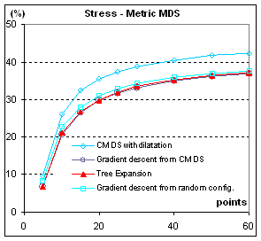
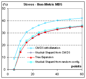
Figure 5: Stress, in %, of configurations from different MDS methods. S= Σ_ij (δ_ij-d_ij)² / Σ_ij dij². All points are from the same population (C=1). When parameters are varied (C>1, clusterscale from 0.0 to 4.0), the stress diminishes when clusters are better separated and augments when there are more clusters with the same separation, but the different methods stay in the same ratio.

Rendering Contingent Data Structure: Figures 6 and 7.

To test how good each MDS algorithm is at rendering accidental structure appearing in data and captured by a SAHN tree, we measured how well clusters defined by the SAHN tree are separated in the final configuration. Using patterns of N² points we adopt the N clusters defined by sectioning the tree at the appropriate level. (Because the tree groups points on the basis of their observed distance, the clusters can contain more or less than N points; they are only constrained to an average of N point per cluster.) The chosen measure of how well these clusters are separated in the configuration obtained by one of the scaling algorithms is the Fisher significance of the groups they define. I.e., from the coordinates of the points in the final configuration, an F-ratio can be computed, and from it a p-value. This p-value reflects the probability that a random configuration would keep the clustered points as well together as the observed configuration does. The p-value is not a perfect measure, in particular it improves when the points that belong to the same cluster get closer to each other, regardless of what their dissimilarity is. By over-gathering the points, one gets a better p-value at the expense of a higher stress; notably, Classical Multi-Dimensional Scaling does just that, because it tends to squash more strongly smaller dissimilarities, which happen to lie more often within the clusters than between them. However, for solutions equivalent in stress, the p-value reflects how well the clusters are separated.

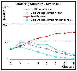
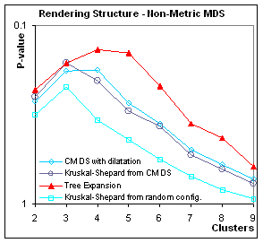
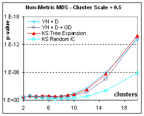
Figure 6: How well is contingent structure rendered? These graphs plot p-value (the significance of the grouping) in function of the number N of clusters (for a total of N² points). When using metric scaling (gradient descent on the dissimilarities), the accidental organization of homogeneous data (all points come from the same Gaussian distribution) is can be preserved by Tree Expansion, but not when other algorithms are used. When using non-metric scaling, Tree Expansion still fares better than other methods, but overall all methods fail to preserve structure.

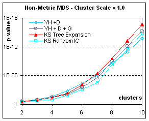
Figure 7: Rendering contingent structure of heterogeneous data: if the data is drawn from different populations, accidental structure is more pronounced and the p-value becomes more significant. Here we show only the non-metric MDS results (metric results are similar). The more separated the population the easier it is to get good final separation from any kind of initial condition; however tree expansion is always the best initial condition. When the scale is only 0.5, good separation only appears for numerous configurations (more than 100 points). With very heterogeneous data (clusters separated by more than one bandwidth), Classical MDS (in this case, applied to dissimilarities) can occasionally give the best p-value, not because it separates clusters better, but because in the same distance-squashing process that causes a higher stress, CMDS brings points of the same cluster closer to their centroid. In all cases, Tree expansion gives a better p-value than Kruskal-Shepard gradient descent from any other initial condition.

Rendering pre-assigned clusters: Figure 8.

Sometimes the grouping of data points is known in advance from extraneous data. For example, clustering could represent the value of a between-subject factor, observed or assigned. In this case the tree-expansion algorithm must be used with a compliant tree, that is, a tree that first organizes the data points inside clusters before it organizes the clusters. With such a tree, expansion will first arrange spatially cluster centroids, then arrange the individual points making up these clusters.

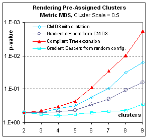
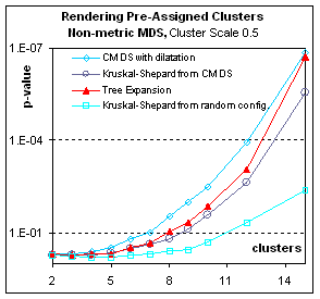
Figure 8: How well are pre-assigned clusters rendered? These graphs plot p-value (the significance of the grouping) in function of the number N of clusters (for a total of N² points). Here the pre-assigned clusters correspond to different populations in the full-dimensional space, such that the centroids of the clusters are distributed with 0.5 times the bandwidth used to distribute points inside clusters around their centroid. The clusters are therefore widely overlapping. Nevertheless, both in the metric and the non-metric case, Multidimensional scaling can render in two dimensions the difference between populations. Expanding the compliant tree is of all gradient descents the most efficient way to render the clusters (In fact it eventually surpasses CMDS in spite of the p-value bias for the latter, at 20 clusters – not shown; p-values for more than 20 clusters could not be computed as they exceeded the double float precision but the F statistic indicated that eventually gradient descent from CMDS also outperforms simple CMDS). If the clusters do not correspond to any difference in spatial repartition (Result not shown) – Cluster Scale=0.0, corresponding to a homogenous population with arbitrary labeling– all p-values are very poor (over .5) but compliant tree expansion is the best of those bad solutions.

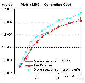
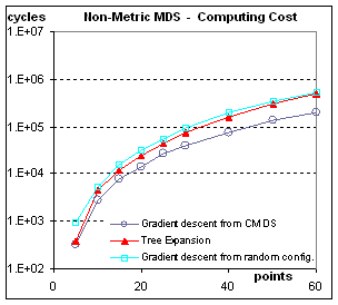
Computational Cost: Figure 9.

One of the worries one might have with the tree expansion method is about the cost of repeating the work of repeatedly organizing almost the same configuration. The results presented in Figure 9 show that this worry is partly justified. For non-metric scaling, tree expansion is about 2.5 times as slow as doing Kruskal-Shepard only once, from the results of CMDS. This does not take into account the lower order costs of building the tree for one algorithm, or of diagonalizing the double-centered dissimilarity matrix for the other algorithm. For metric scaling, tree expansion is actually the cheapest way. This result is counter-intuitive if one thinks in terms of re-doing the work, but makes sense when considering that each expansion stage provides a starting configuration very close to the final configuration for that stage.

Figure 9: Computational Cost. The cost is measured in basic cycles (computing the contribution of one pair of points to one coordinate of the gradient). Even though it is related to the implementation, this cycle count allows to compare the speed of convergence from different initial conditions.

Cost of doing better than Tree Expansion:

If the main focus is on the quality of the configuration obtained, it makes sense to consider the strategy of starting gradient descent repeatedly from many random initial conditions. One may hope that through the force of sheer numbers, a solution will be found that simultaneously lowers stress and renders well the original accidental structure. Tables 1 and 2 present very contrasting results, denying this hope for metric scaling, but keeping the door open for non-metric scaling. Each column presents data from 99 configurations for each of which results from 100 random initial conditions were compared to the result of tree expansion. We show the mean percentage of random initial conditions doing better than tree expansion on stress only, p-value only, and on both simultaneously. To give an idea of the distribution we also show the median configuration and the 5^th centile most favorable to random initial conditions.

Metric MDS %age of RIC trials as good or better than Tree Expansion…	Points in Configuration	5	10	15	20	25	30	40
	Clusters	2	3	4	5	6	6	7
…for Stress only	mean %	69*	26*	21	16	13	12	8
…for p-value only	mean %	75*	42*	17	9	3	3	1
…for both Stress and p-value simultaneously	mean % median % 5^thcentile %	15 0 69	3 0 30	0 0 0	0 0 0	0 0 0	0 0 0	0 0 0

Non-Metric MDS %age of RIC trials as good or better than Tree Expansion…	Points in Configuration	5	10	15	20	25	30	40	50	60	80
	Clusters	2	3	4	5	6	6	7	7	8	9
… for Stress only	mean %	76	32	32	31	37	31	31	28	25	26
… for p-value only	mean %	34	40	38	27	21	25	17	22	18	18
…for both Stress and p-value simultaneously	mean % median % 5^thcentile %	15 4 59	4 0 37	6 0 41	4 0 53	3 0 19	3 0 35	3 0 28	4 0 37	2 0 30	4 0 48

Tables 1 and 2: Comparing Random Initial Condition trials to Tree Expansion. The mean and highest 20-ile of 99 data points, where each time 100 trials were run with different initial configurations and their result compared to the result of tree expansion. In the “both simultaneously” case, we report the mean rather than the median, and also report the 5^th centile, because floor effects quickly intervene: the median for “both” is zero for all number of points. The 5^th centile is the number of random trials, out of 100, doing better than tree expansion in the one-in-twenty situation where that number is the highest. Another remarkable fact is that the probabilities for a random trial of being better than tree expansion for stress, and for p-value, are not independent, but inversely related. This shows that tree expansion strikes a remarkable compromise between both criteria.

* For small configurations the large majority of random initial configuration converges to the same configuration as tree expansion does.

Comments on tables 1 and 2:

For non-metric MDS, random initial conditions results are more frequently equal to or better than tree expansion results. We believe that it is because Non-metric MDS is less demanding than metric MDS (it only tries to respect the order of the original dissimilarities) and that therefore the process of organizing intermediary stages of expansion is stunted by being stopped as soon as intermediary dissimilarities are “good enough”.
For metric MDS, percentages of random initial conditions that yield as good a result on either stress or p-value steadily decrease with the number of points in a pattern.
For non-metric MDS, the percentage of random initial conditions that yield as good a result on either stress or p-value is almost constant, and confirm common wisdom that 4 or 5 random trials are usually enough to get a good value of stress.
For both metric and non-metric MDS, the distribution of results is very skewed. The medians are much lower than the means; i.e., there are a few of the 99 configurations for which many random conditions will do fairly well, but for the large majority they do very poorly.
For metric MDS, the probabilities of being better on Stress and being better on p-value are not independent; if they had been the mean on both would be a product of the means on each. In fact the percentage of simultaneous success is much lower than can be predicted from the percentages of being better on one count only. This suggests that for metric MDS there has to be a trade-off between both properties. For this trade-off, both tree expansion and gradient descent from classical MDS strike a much better compromise than random conditions can hope to reach; within that compromise, tree expansion favors p-value and descent from classical MDS favors stress.
For non-metric MDS, the probabilities of being better on Stress and being better on p-value seem to be fairly independent.

Example: Multidimensional Scaling of Cereal data:

As an example, several scaling techniques were applied to the data offered for the 1993 ASA Statistical Graphics Exposition (http://lib.stat.cmu.edu/datasets/1993.expo/cereal). The data has 13 fields, the first two being categorical: cereal manufacturer, and hot or cold cereal. “Hot or cold” was encoded as +1 or -1. Thereafter, all 12 numerical fields were normalized to a mean 0 and a variance 1, and between-cereal distance was computed in the resulting 12-dimensional Euclidian space. Two approaches were taken to this data: first, by clustering according to the cereal manufacturer, and second, by building a SAHN Tree (centroid-based). Clustering by manufacturer did not yield any significant classification – p values for all methods were greater than .5. For the second approach, all scaling methods were able to cluster the points decently, but tree expansion did so much better. Table 3 summarizes the quantitative results, and Figure 10 shows the resulting configurations.

	Metric			Non-Metric (Kruskal-Shepard)
	Stress	p-value	cost index	Stress	p-value	Cost index
Tree Expansion	23.8 %	3.9 e-6	127,769	18.4 %	1.7 e-6	561,814
CMDS + D with GD or KS	23.4 %	1.8 e-3	335,566	18.5 %	1.1 e-5	154,154
CMDS + D without gradient descent or Kruskal-Shepard descent.	32.7 %	2.0 e-4	n/a	29.8 %	2.4 e-4	n/a
non weighted Tree Expansion	23.2 %	1.9 e-4	498,118	18.4 %	1.9 e-6	692,216
Circular Initial Configuration (better than random on most counts)	24.0 %	1.9 e-3	1,555,708	20.2 %	2.2 e-3	492,107

Table 3: Stress, p-value, and computing cost for scaling configurations of the cereal data, obtained ether by Tree Expansion or by gradient descent (or Kruskal-Shepard) completing CMDS.

Symbol

Ad-hoc title

and description

Cereals in that cluster

Fruits and Nuts

fairly rich in protein and fat

but low in slow carbs

Almond_Delight R

Crispy_Wheat_&_Raisins G

Life Q

Quaker_Oat_Squares Q

Clusters G

Raisin_Nut_Bran G

Cracklin'_Oat_Bran K

Great_Grains_Pecan P

Muesli_Raisins,_Dates,_&_Almonds R

Muesli_Raisins,_Peaches,_&_Pecans R

100%_Natural_Bran Q

Fruits and Bran

heavier – densest cereals

Just_Right_Fruit_&_Nut K

Total_Raisin_Bran G

Post_Nat._Raisin_Bran P

Raisin_Bran K

Fruitful_Bran K

Fruit_&_Fibre_Dates,_Walnuts,_and_Oats P

Oatmeal_Raisin_Crisp G

Basic_4 G

Nutri-Grain_Almond-Raisin K

Mueslix_Crispy_Blend K

Classic Cereals

high slow-carb content,

hi sodium

Just_Right_Crunchy__Nuggets K

Total_Corn_Flakes G

Total_Whole_Grain G

Product_19 K

Cheerios G

Special_K K

Corn_Chex R

Rice_Krispies K

Corn_Flakes K

Rice_Chex R

Kix G

Puffed and agglomerated

low fat, sugar and fiber content,

medium slow carb content

Puffed_Rice Q

Puffed_Wheat Q

Frosted_Mini-Wheats K

Strawberry_Fruit_Wheats N

Raisin_Squares K

Shredded_Wheat_'n'Bran N

Shredded_Wheat_spoon_size N

Shredded_Wheat N

Multi-Grain_Cheerios G

Wheaties G

Bran_Chex R

Wheat_Chex R

Crispix K

Triples G

Double_Chex R

Nutri-grain_Wheat K

Grape_Nuts_Flakes P

Bran_Flakes P

Grape-Nuts P

Hot cereals

Cream_of_Wheat_(Quick) N

Maypo A

Quaker_Oatmeal Q

Pure Bran

low calories, low slow carbs,

low sugar, high potassium

100%_Bran N

All-Bran K

All-Bran_with_Extra_Fiber K

Fancy cereals

more sugar,

lower shelf placement

_Crisp P

Smacks K

Apple_Jacks K

Corn_Pops K

Froot_Loops K

Lucky_Charms G

Cocoa_Puffs G

Count_Chocula G

Trix G

Fruity_Pebbles P

Honey-comb P

Cap'n'Crunch Q

Honey_Graham_Ohs Q

Cinnamon_Toast_Crunch G

Apple_Cinnamon_Cheerios G

Honey_Nut_Cheerios G

Nut&Honey_Crunch K

Wheaties_Honey_Gold G

Golden_Grahams G

Frosted_Flakes K

Table 4: The clusters defined by a section of the SAHN tree at the 7^th level. The cluster titles are descriptive, and the comments below the titles summarize the main common properties, observed manually, for the cluster members.

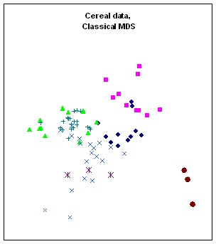
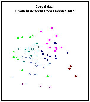
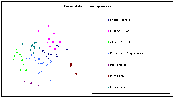
Figure 10: Rendering the cereal data by different algorithms: a. classical scaling (Young-Torgerson reduction); b. classical scaling followed by a gradient descent to minimize residual square error; c. expansion of the SAHN tree, applying gradient descent to adjust the configuration every time a point is split. Notice how Classic cereals (rendered by green triangles) are dispersed when gradient descent takes classical scaling as an initial configuration, because that cluster overlaps another one which is more compact. This is a “mountain pass” effect, as is probably the isolation of two “dark diamond” points inside the cluster of “purple squares”. In contrast, the tree expansion is relatively free of such effects.

Ramifications:

The computations described here have just begun to explore a large set of possible variants. Only one type of tree was used (binary SAHN centroid tree). It is likely that different types of trees are more efficient for different data sets. Tree expansion does not have to be restricted to expanding binary trees; one can easily figure extensions of the method using any kind of tree. When computing time is not critical, we suggest expanding several candidate trees.

In fact expanding a non-binary tree is equivalent to skipping a few stages of intermediary gradient descent in expanding a binary tree. Such a strategy can be employed deliberately if computing power is at stake, or simply if it is known from the structure of the data that fewer stages of expansion are sufficient. The archetypical example would in the situation of rendering known clusters, to first use tree expansion (or another algorithm) to place the cluster centroids, and then in one stage replace all centroids by the points of the corresponding cluster.

One variant we considered and which occasionally yielded better results than reported for the main variant was not to consider the differences in centroid mass during the gradient descents.

The simulations were limited to 2-D configurations, even though the algorithm applies also for uni-dimensional scaling (UDS). The uniqueness of UDS stems from two peculiarities: first, the local minima problems of gradient descent are much worse in one dimension, and second, being in one dimension only facilitates a combinatorial approach (Defays 1978). We believe that for UDS, the best use of tree expansion will require its combination with heuristic combinatorial techniques. The simplest example is to confine heuristic exploration to the group of permutations along the tree (the group generated by all transpositions of two direct offspring of the same node), which is a subgroup of only 2^N out of the N! permutations of all points. For large data sets, one could explore all tree-defined permutations only a few levels down from the current level. For example, when expanding from four point to five, rather than select the immediate best configuration of 5 points (best out of two choices), one could consider all 16 potentially resulting configurations of 8 points, then finalize the choice of the five point configuration to the configuration leading to the lowest 8–point stress. In the application of tree expansion, as in other matters, UDS deserves a fully independent treatment, because of the facility with which it allows combinatorial schemes, and because of the connections between UDS and tree-building.

Even for 2-D or 3-D configurations, tree expansion can be applied in conjunction with some random exploration of initial conditions space. For example, one can replace the early part of expansion, placing the first P points by random exploration, and then expanding those nodes into a full configuration by normal tree expansion. The configuration obtained by tree expansion at various steps can be used as one of the strains for a genetic algorithm—in other problems requiring gradient descent, genetic algorithms (Goldberg 1989) have been efficient ways of cutting down the complexity of random exploration (Nolfi, Elman et al. 1994).

Tree expansion can also be combined with heuristic search by applying the heuristic at the level of tree-building. For a tree built bottom-up (as SAHN trees are), some agglomeration choices are obvious and some are not. By combining all the close calls into a family of alternate trees, one creates as many possible ways of seeking an optimal configuration.

Finally, Tree Expansion may be combined with other strategies that can bias the rendering in favor of particular clusters. The most prominent of these is to weight the contribution of different pairs of points in the gradient, in order to favor either the within-cluster or the between-cluster distances. Because the good properties of tree expansion originate from setting a proper initial configuration, all others methods that do not rely on particular initial conditions should benefit from being used in conjunction with tree expansion.

Summary and conclusion:

This article suggests a new type of initial configuration to use for gradient descent multidimensional scaling algorithms such as Kruskal-Shepard. Using a binary hierarchical tree of the points to scale, one can expand that tree in the final space, starting with the root and repeatedly replacing each node by its two successors; at each expansion one uses the gradient descent again to reshape the configuration. Compared to applying gradient descent to the result of classical scaling, tree expansion is tidier, and more apt at keeping together points belonging to the same cluster. In particular, when the clusters tend to overlap, tree expansion can find significant representations whereas other methods fail.

Besides our main result, the explorations made in this paper shed light on basic differences between metric and non-metric MDS, that users should keep in mind when they have a choice between both methods. Metric MDS is more demanding; by doing gradient descent on the dissimilarities themselves it strives for perfection. In comparison, non-metric MDS only strives for distances in the right order. In the scope of our simulations, these differences twice caused finer results from metric MDS: first in that contingent structure of homogeneous data can be rendered significantly by metric MDS (Figure 6), but not by non-metric; and secondly, in the trade-off that metric MDS forces between finding a good stress and rendering structure (Table 1). The goal of the Kruskal-Shepard algorithm is as much finding the psychometric function relating dissimilarities to distances as it is to find those distances. To make the Kruskal-Shepard algorithm as demanding on the distances as metric MDS is, one would need to add constraints on the shape of the psychometric function, constraints that would make further demands than the simple monotonous regression. In fact, there lies a continuum of algorithms from metric MDS, where the psychometric function is imposed to be identity, to the Kruskal-Shepard algorithm, where it can take any monotonous shape. For this reason, the choice between metric and non-metric MDS –or other intermediary algorithms—should be dictated not by convenience, but by what one expects the psychometric function to be.

The results presented here should be taken as the floor, not the ceiling, of tree expansion efficiency. Firstly, there is no guarantee that type of tree used here was the best for the testing data. Secondly, the data might not be the most difficult for the classical methods that we compared tree expansion to. In our results, metric scaling of the dissimilarities followed by gradient descent fare quite well, always better than random initial conditions. This is not the case for all possible problems; for example Arabie and Boorman (1973, p.160) report scaling configuration representing partitions for which CMS followed by non-metric gradient descent fared worse than random initial conditions. In contrast to the metric scaling of similarities, tree expansion is a robust process, which we expect to degrade well with problem difficulty, its weakness being only the representative quality of the tree.

By using tree expansion, classical metric and non-metric scaling becomes a field of application of hierarchical clustering, and the large existent corpus of clustering algorithms must be tested to find out which tree are the best candidates for expansion.

Acknowledgements:

The author wishes to thank for their help Professor David Kirsh, Daniel Bauer, and John Hershey. This work was funded by a grant from France Telecom.

Reference:

Arabie, P. and S. A. Boorman (1973). "Multidimensional scaling of measures of distance between partitions." Journal of Mathematical Psychology 10: 148-203.

Arabie, P., L. J. Hubert, et al. (1996). Clustering and Classification. Singapore, World Scientific.

Cox, T. F. and M. A. A. Cox (2001). Multidimensional Scaling. Boca Raton, Chapman & Hall.

Defays, D. (1978). "A short note on a method of seriation." British Journal of Mathematical Statistical Psychology 31: 49-53.

Goldberg, D. E. (1989). Genetic Algorithms, in search, Optimization and Machine Learning. Readin, Mass., Addison-Wesley.

Gordon, A. P. (1996). Hierarchical Classification. Clustering and Classification. P. Arabie, L. J. Hubert and G. de Soete. Singapore, World Scientific. 1: 65-121.

Kruskal, J. B. (1964). "Multidimensional Scaling by Optimizing Goodness of Fit to a Nonmetric Hypothesis." Psychometrika 29(1): 1-27.

Kruskal, J. B. (1964). "Nonmetric Multidimensional Scaling: a Numerical Method." Psychometrika 29(2): 115-129.

Kruskal, J. B. (1977). The relationship between Multidimensional Scaling and Clustering. Classification and clustering. J. van Rezin. Reading, MA, Addison-Wesley: 17-44.

Lingoes, J. C. and E. E. Roskam (1973). "A mathematical and empirical study of two multidimensional scaling algorithms." Psychometrika Monograph Supplement 38.

Nolfi, S., J. L. Elman, et al. (1994). "Learning and evolution in neural networks." Adaptive Behavior 3(1): 5-28.

Press, W., S. Teukolsky, et al. (1992). "Numerical Recipes in C, second edition."

Shepard, R. (1958). "Stimulus and response generalisation: tests of a model relating generalization to distance in psychological space." Journal of Experimental Psychology 55(6): 509-523.

Shepard, R. N. (1962). "The Analysis of Proximities: Multidimensional Scaling with an Unknown Distance Function. I." Psychometrika 27(2): 125-140.

Shepard, R. N. (1962). "The Analysis of Proximities: Multidimensional Scaling with an Unknown Distance Function. II." Psychometrika 27(3): 219-246.

Torgerson, W. S. (1952). "Multidimensional scaling: 1. Theory and method." Psychometrika 17: 401-419.

Young, G. and A. S. Householder (1938). "Discussion of a Set of Points in Terms of Their Mutual Distances." Psychometrika 3(1): 19-22.