|


Classification
 |
| Figure 1: The Grail of Classification: to be able to capture conceptual structure in a visually striking way. |
When trying to visualize the proximity structure of a high dimensional pattern, one frequently has to choose between clustering into a hierarchical tree, or projecting the pattern in two or three dimensions. Conventional wisdom considers that multi-dimensional scaling (projection) is good at representing the big picture, whereas hierarchical clustering handles local details more faithfully. Ideally, one would want a low-dimensional configuration rendering both the global and local properties; such that, for example, if one drew between the final points a hierarchical tree obtained from the original data, this tree would appear simple and related branches would stay next to each other. Our research adapts existing scaling algorithms to create such tree-friendly configurations.
Why Existing Scaling Strategies Deal Poorly with Local Structure
 |
|
Figure 2 illustrates two problems: |
|
| 1. | Because it lies parallel to an eigenvector pruned by the CMDS, the distance between B and C has been ignored. In contrast, the distance between A and the other points is almost conserved, because it is almost collinear to the eigenvector preserved by the CMDS. |
| 2. | The projection ignores the arc, so that even though B and C are both at the same distance from A, their projection gets closer than that distance. |
Instead of relying exclusively on the one-shot CMDS procedure, one can optimize the placement of the points by gradient descent, but this approach is plagued by local minima |
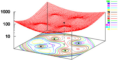 |
| Figure 3: Local minima in a metric energy landscape. |
When scaling the five points (4, 4, 0), (4,-4,0), (-4,4,0), (-4,-4,0) and (1,1,7), CMDS projects the latter in the plane Z=0, onto the point (1,1,0) shown in grey. This graph shows a 2-D section of a 10-variable function: the sum of residuals landscape, by fixing the coordinates of the 4 points that were already in the plane (“the base”) and showing the sum of residuals for different locations of the 5th point. For moving the grey point only, there are at least five local minima: four located outside the base and one about (-1, -1, 0). In fact, this latter point is where gradient descent takes the grey point, but it is not the absolute minimum.
In order to jointly minimize stress and render the cluster structure, we propose to apply gradient descent (or Kruskal-Shepard) repeatedly to a growing configuration, obtained by expanding the hierarchical tree. This is illustrated by Figure 4 in which the hierarchical tree and successive configurations are shown bide by side. Prior to using this algorithm, one needs the dissimilarity matrix at all stages of expansion. If the tree has been constructed from a SAHN algorithm these dissimilarities are already available, otherwise they have to be computed in a one-sweep forward pass. Given these dissimilarities, the algorithm is to:
| 1. | Position a starting configuration: |
| 2. | Expand the tree: |
| 3. | Make a final adjustment down to the desired accuracy. |
 |
| Figure 4: MDS by Tree expansion |
In the left column, the SAHN tree clustering 9 color samples used by Roger Shepard in misidentification judgments. The 9 circles at the bottom are the colors used experimentally; higher level tree nodes received interpolated RGB values. The top of the tree (top node and its immediate offspring) is truncated.
In the right column, successive 2-D configurations obtained by tree expansion. The 3-point configuration is an exact CMDS scaling. Subsequent configurations (4 to 9 points) are obtained by Kruskal-Shepard, using as initial condition the previous configuration in which one point is replaced by its two contributors. The point chosen is the current highest tree node, it will be replaced by the two tree nodes that it consists of, and those two nodes start with their parent’s location – it is the Kruskal-Shepard algorithm that pulls them apart.
On both sides, a blue arrow points at the node about to be split. In the right panel, as the pattern is expanded from 3 points to the full 9 points, we see that some expansions require more reorganization (e.g., from 6 to 7 points) but there is no reversal of relative positions.
Example: Clustering the American Statistical Association Sample Data on Cereals
 |
| Figure 5: The American Statistical Association published in 1993 a test bed for MDS algorithms, consisting of 13-dimensional data on 77 types of breakfast cereals. |
This cereal data is rendered here by different algorithms: a. classical scaling (Young-Torgerson reduction); b. classical scaling followed by a gradient descent to minimize residual square error; c. expansion of the SAHN tree, applying gradient descent to adjust the configuration every time a point is split. Notice how Classic cereals (rendered by green triangles) are dispersed when gradient descent takes classical scaling as an initial configuration, because that cluster overlaps another one which is more compact. This is a “mountain pass” effect, as is probably the isolation of two “dark diamond” points inside the cluster of “purple squares”. In contrast, the tree expansion is relatively free of such effects.
|
|